Spatial Search Algorithms: Querying Millions of Points Instantly

When processing and displaying spatial data at scale, few concepts are as useful as a spatial index. Spatial indexing algorithms organize geometry so that queries can avoid scanning the entire dataset. Typical queries include:

Return every building in an area
Find the 1,000 gas stations nearest to a point

Even with millions of objects, a spatial index can return results in milliseconds. It underpins spatial databases such as PostGIS, itself a core component of many GIS platforms. One server-side application is processing telemetry: map-matching millions of GPS speed samples to a road network to generate live traffic data. Client-side uses include placing map labels in real time and hit-testing map objects under the pointer.

Mapbox developers have built several efficient JavaScript spatial-search libraries, including rbush, rbush-knn, kdbush, and geokdbush. This article explains the principles behind them.

Spatial Query Types

Two fundamental query types underlie many geometry and GIS problems: nearest-neighbor queries and range queries.

K Nearest Neighbors

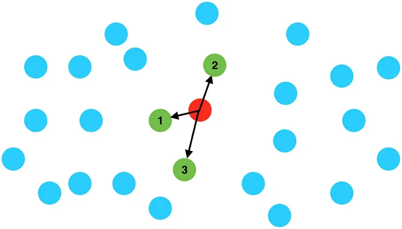
The three nearest neighbors of a query point

Given thousands of points, such as city locations, how can we retrieve those nearest to a query point? A direct method is to:

Calculate the distance from the query to every other point.
Sort all points by distance.
Return the first K.

This is acceptable for a few hundred points but becomes impractical with millions.

Range and Radius Queries

How can we retrieve every point inside:

A rectangle, for a range query?
A circle, for a radius query?

Again, scanning every point fails when the database is large and must serve thousands of queries per second.

How Spatial Index Trees Work

At scale, points must be organized into a spatial index. Data usually changes far less often than it is queried, so the up-front indexing cost pays for fast subsequent searches.

Almost every spatial data structure relies on the same principle: branch and bound. Data is organized into a tree, and any branch that cannot satisfy the query is discarded immediately.

R-tree

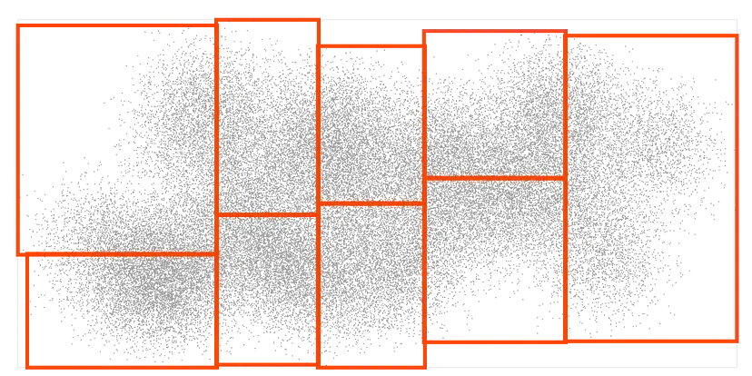
Begin with a set of points and group them into nine bounding boxes containing roughly equal numbers of points:

Then subdivide each box into nine smaller boxes:

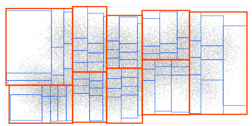
Repeat until each leaf box contains at most nine points:

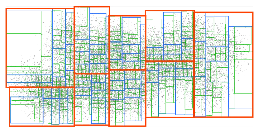
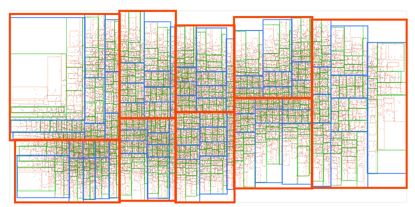
The result is an R-tree, probably the most common spatial data structure. It is used by modern spatial databases and many game engines.

An R-tree can index rectangles as well as points, and those rectangles can bound arbitrary geometry. The structure also extends to three or more dimensions, although the discussion below uses 2D points.

K-d Tree

A k-d tree is another popular spatial structure. Instead of grouping points into several regions at each level, it splits them around a median into two halves—left and right or above and below—alternating between the x- and y-axes:

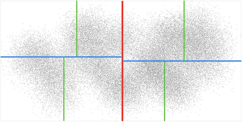
Compared with an R-tree, a k-d tree generally indexes points rather than rectangles and is less suited to insertion and deletion. It is much simpler to implement and extremely fast. Both structures partition data into axis-aligned nodes, so the search algorithms below apply to both.

Range Queries in a Tree

A typical spatial tree looks like this:

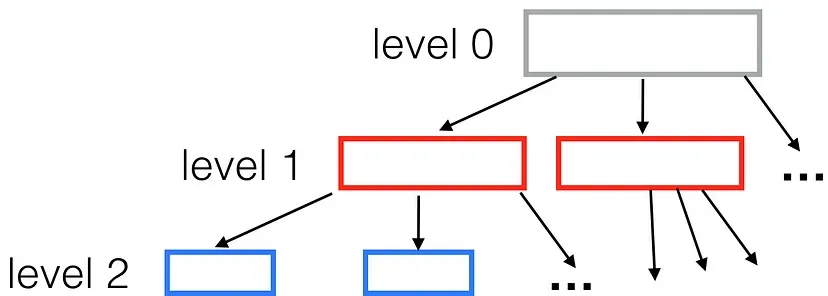
Each node has a fixed number of children—nine in this example. For one million points, the height is ceil(log(1000000) / log(9)) = 7.

A range query descends from the root while ignoring every node whose bounds do not intersect the query rectangle. A small query intersects only a few regions at each level. Instead of one million comparisons, the search may require roughly 60 box tests—7 × 9 = 63—about 16,000 times fewer than a linear scan.

In asymptotic terms, an R-tree range query averages O(K log N), where K is the output size, compared with O(N) for a linear scan.

Nine is a useful default node capacity. In general, larger nodes make index construction faster but queries slower; smaller nodes reverse that tradeoff.

K-nearest-neighbor Queries

Nearest-neighbor search is more subtle. Which nodes should be explored for a given query point? A radius query is not enough because the necessary radius is unknown and the nearest point may be far away. Repeating queries with increasing radii is inefficient.

The solution uses a priority queue, which maintains ordered candidates and efficiently removes the smallest. Return to the R-tree example:

Boxes nearer to the query are more likely to contain its nearest points. Start at the root and enqueue the top-level boxes ordered by their minimum possible distance to the query:

Remove the nearest box, “open” it, and insert all of its child boxes back into the same ordered queue.

First- and second-level nodes in one queue

Continue opening the nearest box and enqueueing its children. When the nearest queue item is an actual point, it is guaranteed to be the nearest point. The next point removed is the second nearest, and so on.

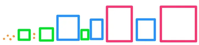
Nodes and points from all levels mixed in one priority queue

The guarantee follows from the lower bound stored for every unopened box: no point inside it can be closer than the box itself. A point at the head of the queue is therefore no farther than anything hidden in the remaining boxes.

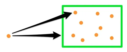
Distance to a box is a lower bound for every point inside it

If the tree is balanced, only a small number of boxes need to be opened; most branches remain untouched, making the algorithm extremely fast.

Custom Distance Metrics for kNN

This box-expansion method is flexible. It only requires a lower bound between the query object and every object inside a box. If such a bound can be defined for a custom metric, the same algorithm applies.

For example, it can find the K points nearest to a line segment rather than to another point:

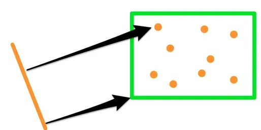
Segment-to-box distance as a lower bound for points inside the box

Replace point-to-point and point-to-box distances with segment-to-point and segment-to-box distances. The 2D concave-hull library Concaveman uses this technique to generate outlines such as:

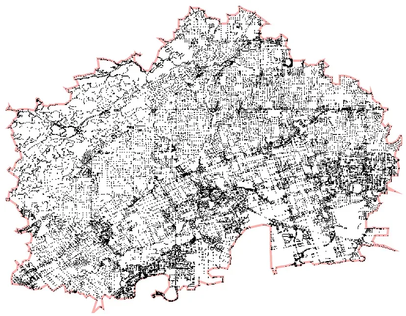
The algorithm begins with a fast convex hull, then progressively bends its boundary inward by connecting nearby interior points:

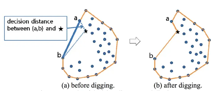
In the paper that proposed this concave-hull method, finding the nearest eligible interior point for every boundary edge — the candidate points for carving into the hull — was a time-consuming step, and developing a faster approach was left as future work.

The challenge is that with many data points, searching for interior points near each boundary edge becomes very expensive. Future research could focus on improving the search itself, for example by using a more efficient spatial index such as a k-d tree or R-tree to speed up the nearest-point lookups and improve overall performance.

Further Spatial-index Improvements

R-trees and k-d trees are sufficient for many small or straightforward datasets. More demanding cases can consider:

Adaptive node splitting: adjust splits to the observed distribution to reduce tree height and bounding-box overlap.
Optimized custom metrics: derive cheaper lower-bound calculations for queries such as segment-to-box distance.
Better index packing and compression: reduce memory use while preserving query throughput, especially for static indexes.