Implementing Kriging Interpolation, Part 1: The Mathematics

This article began as a major course project during my third year at university and was originally published on CSDN. I put a great deal of effort into it, so I decided to preserve it here.

Kriging is relatively complex, but it can produce high-quality interpolation results. Implementing it in code requires a detailed understanding of the calculations involved.

Performing Kriging in ArcGIS

Import Point Data

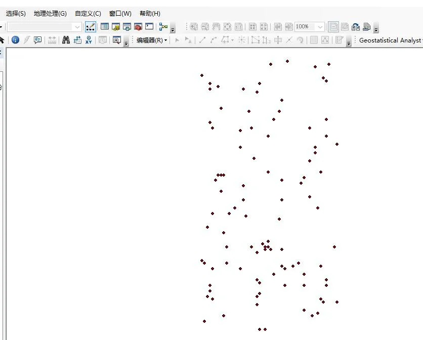
Importing point coordinates and elevation values

Choose Geostatistical Wizard from the Geostatistical Analyst toolbar. If the toolbar is not visible, right-click an empty area of the toolbar region and enable Geostatistical Analyst.

Select the Data

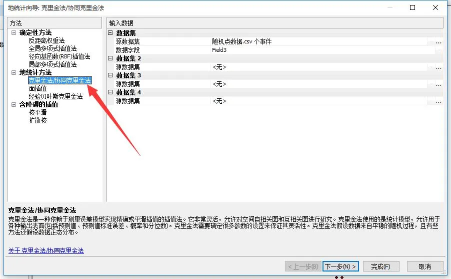
Choose Ordinary Kriging

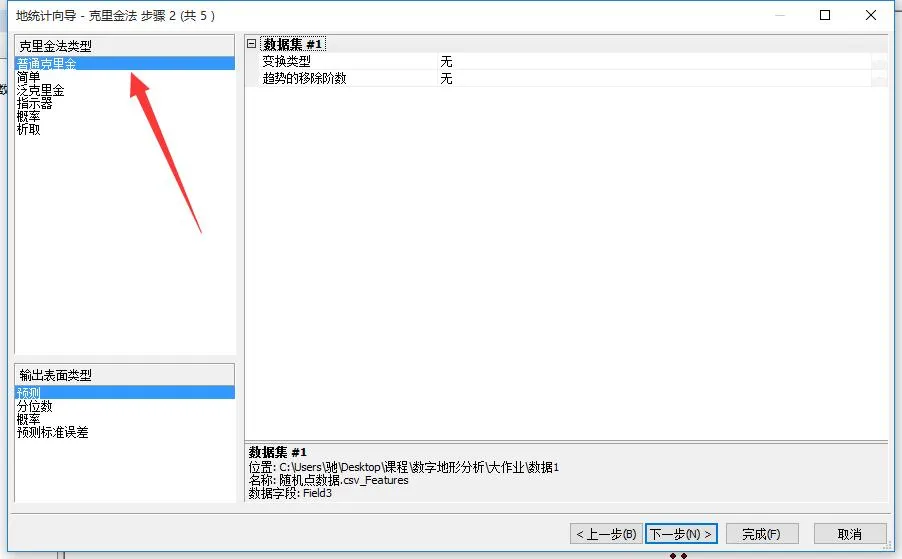
Model-fitting Interface

This screen is important and corresponds to the concepts described in the ArcGIS documentation. The fitted curve in the upper-left corner is what the C# implementation will reproduce, and the plotted points must also be calculated.

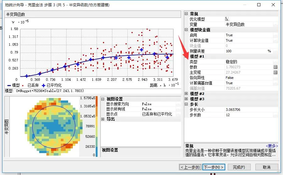
Inspect the Variogram Model Types

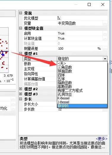
Open the Type menu to choose among spherical, exponential, Gaussian, and other models. Selecting a different type changes the fitted curve on the left. The ArcGIS documentation describes each model.

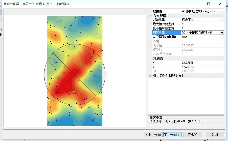
View the Interpolation Result

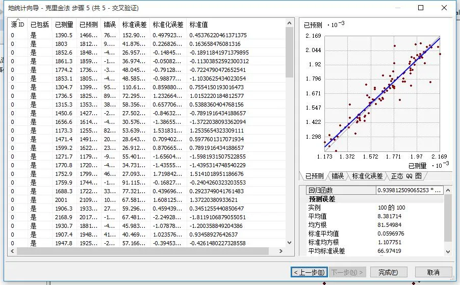
The interpolation result after selecting a model

Error Analysis

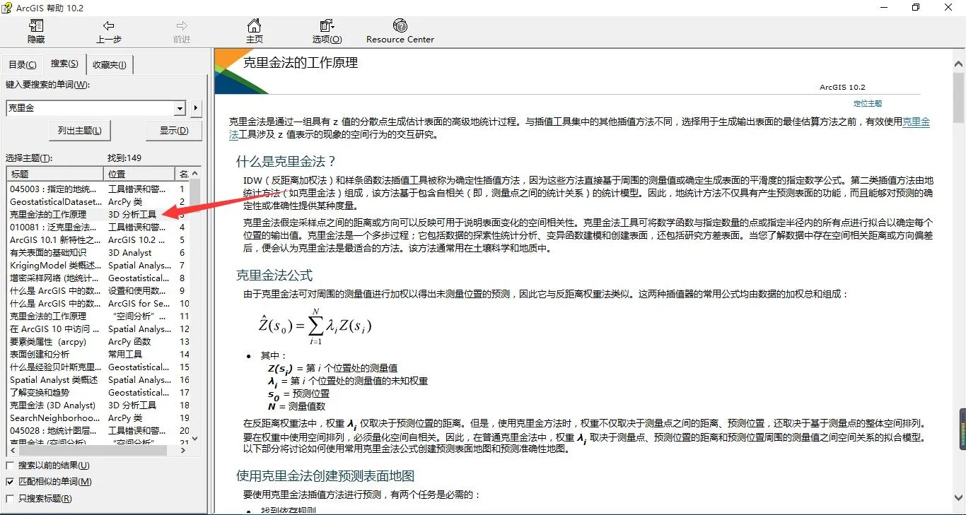
Understanding the ArcGIS Kriging Documentation

Open the ArcGIS help, search for “kriging,” and select “How Kriging works.”

Calculate Pairwise Semivariance

The formula is $Semivariogram(distance_h) = {1\over2} * (value_i - value_j)^2$ , where $distance_h$ is the distance between points $i$ and $j$ and becomes the x-coordinate. The calculated semivariance becomes the y-coordinate.

With 100 points, calculating semivariance between every point and the other 99 produces a large amount of data, including duplicate pairs, and makes fitting inefficient. The documentation recommends reducing the results by distance bins—for example, calculating a mean for 0–10, 10–20, 20–30, and so on.

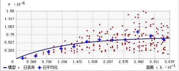
This produces the points shown below: red points are the original pairwise results, and blue points are the bin means.

Fit the Points to Obtain the Range and Sill

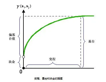
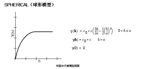
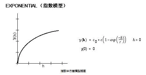
The model is fitted primarily to the blue points. In the equations, $c_0$ is the nugget, $c$ is the partial sill, and $a$ or $r$ is the practical range. The nugget $c_0$ is commonly assumed to be zero in this fitting process.

Spherical Model

Exponential Model

Gaussian Model

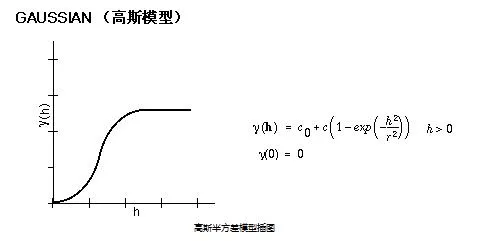
Assuming $c_0=0$ , the spherical equation has three unknowns, whereas the Gaussian and exponential models have two. Because the fitting process must be implemented in C#, I chose the simpler exponential model:

r{(h)} = \begin{cases} c_0+c*(1-e^{{-h}\over r}), & h>0 \\ 0, & h=0 \end{cases}

Fitting yields $c$ and $r$ , producing a semivariogram model that can be used in the interpolation step.

Estimate the Value at an Unknown Point

The ArcGIS help did not describe the remaining calculation in detail, so I obtained the procedure from a competition PDF. Let $r_{(h)}$ be the fitted model above, and let $h$ be the distance between points $i$ and $j$ .

Define $c_{ij}=c-r(h_{ij})$ for constructing matrix $K$ and vector $D$ . Matrix $K$ is calculated from the known sample points:

K= \begin{bmatrix} c_{11}& c_{12} & \cdots\ &c_{1n} \\ c_{21}& c_{22} & \cdots\ &c_{2n} \\ \cdots\ & \cdots\ & \cdots\ & \cdots\ \\ c_{n1}& c_{n2} & \cdots\ &c_{nn} \\ \end{bmatrix}

Vector $D$ contains $c_{ij}$ between the unknown location and every known point:

D= \begin{bmatrix} c(x_1,x) \\ c(x_2,x) \\ \cdots\ \\ c(x_n,x) \\ \end{bmatrix}

Matrix $K$ and vector $D$ yield vector $\lambda$ , where $\lambda(i)$ is the weight assigned to known point $i$ : $\lambda=K^{-1}D$ .

The elevation at $x_0$ is then calculated as $Z(x_0)=\sum_{i=1}^n\lambda_i*Z(x_i)$ , where $Z(x_i)$ is the elevation at known point $i$ .

This estimates the elevation at one unknown point. Matrix $K$ is constant for the same set of samples, so estimating additional locations only requires recalculating vector $D$ .